Figure 1
Welcome to the MISTIC Tutorial!
In the next pages we will use an example case study to help you load data, submit the job and then analyze and visualize the results.
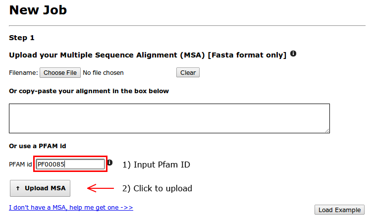
We will be using the Thioredoxin Pfam protein family (PfamID: PF00085). First, we need to upload the Multiple Sequence Alignment (MSA) of this protein family, which in this case will be retrieved from the Pfam Database.
Input "PF00085" in the last box and click on "Upload MSA". The MSA will be downloaded and scanned for formatting errors. If format is correct, new sections of the webpage will become available.
| | |
Figure 1 |
Next, we will specify which sequence from the alignment we just uploaded, is our sequence of interest. This will allow us to use a PDB structure to be mapped to this sequence.
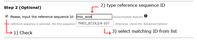 | |
Figure 2 |
A PDB structure needs to be supplied in order to be aligned to the reference structure. It can be uploaded by the user or using a PDB ID, it will be automatically downloaded from the PDB database.
After it is uploaded, the webpage asks to specify which chain will be used.
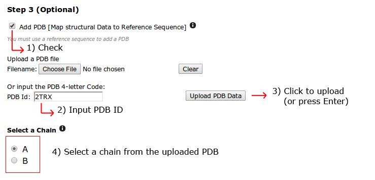 | |
Figure 3 |
Finally, an email address may be supplied if email confirmation of job completion is preferred. The identifier is also optional but encouraged as it will help you identify your job when multiple ones are submitted (or when searching your inbox).
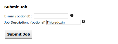 | |
Figure 4 |
A summary of the selected data for submission is shown to check for any errors. Once ready, click on "Submit Job" and wait until calculations are done
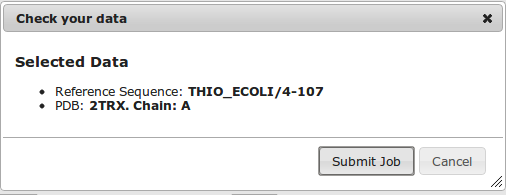 | |
Figure 5 |
The results screen will loook very similar (due to layout calculations) to the one in figure 6. The submitted data is shown and available at the header, followed by the mutual information Circo, and network representations.
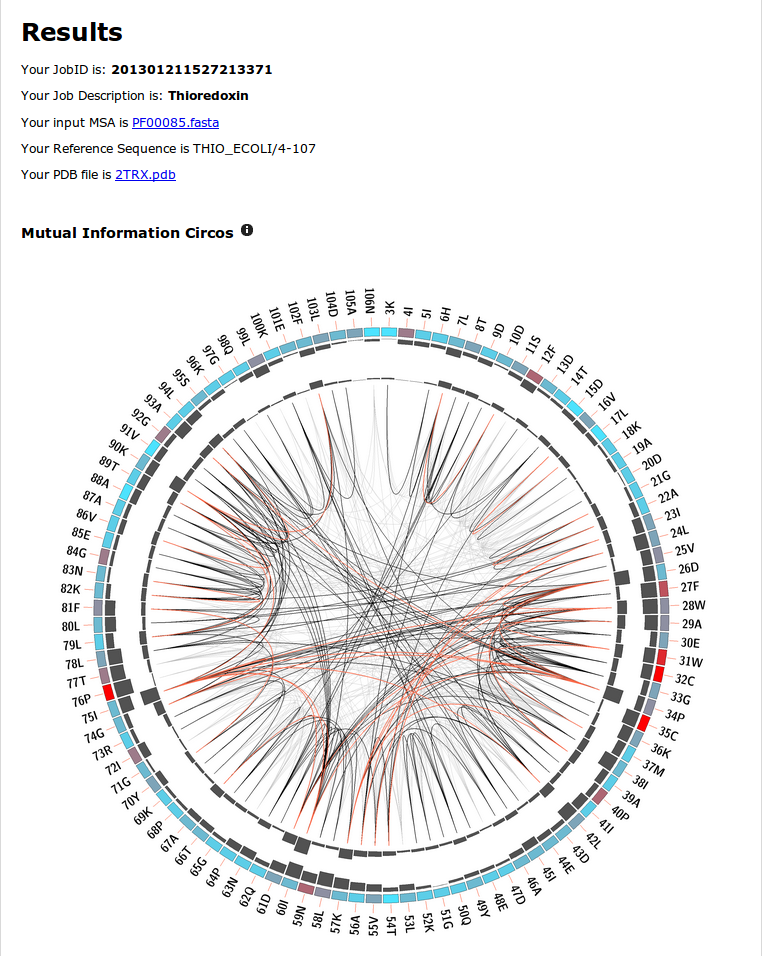 | |
Figure 6 |
You can see there are 3 regions that are slightly more informative than others, as they involve more covariated pairs. These regions are from position 24 to 38, 57 to 61 and 75 to 80. You can identify them by looking at the cumulative and proximity MI histograms, facing outwards and inwards respectively.
Although this example is not an easy one to interpret, you will encounter other cases where interesting regions are more intuitively found using a circos representation.
Scrolling to the end of the results, after the static network images, you will find a dropdown menu with different networks.(Figure 7)
Default network is the one that contains the top 500 MI edges. This is mainly for performance issues, as more edges will make the network bigger, and your browser may crash. If you feel confident your computer (and browser) is able to cope with bigger networks, you can choose to use the complete MI network for the rest of the tutorial.
Once selected, please click on 'Show Interactive Network'
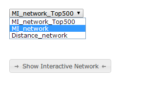 | |
Figure 7 |
You will find a network and a right panel with different tabs
The network is completely interactive and clickable. Try selecting a node, or several nodes by click-dragging your mouse around them.
For the selected nodes, information will be displayed on the right panel, in the 'Nodes' tab
A table with the attributes for each node is displayed, such as conservation score, cumulative MI and proximity MI values
Below, logo representations will show up. If only one node was selected, an histogram showing relative aminoacid frequencies will be displayed. This frequencies correspond to the MSA column that the selected node represents.
 | |
Figure 8 |
The resulting network is quite complicated, with too many edges to be easily viewed. We can reduce the amount of MI edges by filtering the weakest MI edges.
First, go to the filter tab (Figure 9). You will find two kinds of filters, edge filters and node filters.
To hide the weakest MI edges, just move the left end of the slider to the right. The number of MI edges will start to decrease. Keep moving the slider until only the best 20 edges remain.
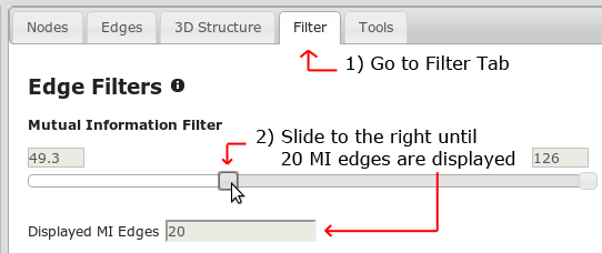 | |
Figure 9 |
After this, click on the 'Uptade Layout' button at the bottom of the tab. The resulting network should look similar to Figure 10.
In order to select the biggest subnetwork, the easiest way to do this is to select a node contained in it, and then click 'Get Associated Maximal Subnetwork'. The algorithm 'travels' from the selected node along its edges to other nodes, and so on, until all connected nodes are visited.
A simplified version is also available, which gets the 'First Neighbours' of a node.
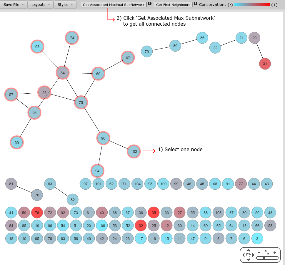 | |
Figure 10 |
Finally, go to the '3D Structure' tab (Figure 11). The PDB structure will load and display on the Jmol Applet. You should see in red the residues that are mapped to the selected nodes on the network. In some browsers it is necessary to refresh the view in the Jmol applet each time the tab is changed.
Now, lets select the catalytic residues for the thioredoxin structure. These are residues 32 and 35. Input in the box (3) the node labels separated by a comma (32,35) and click on select. They should now be marked in red in the structure. Then, save the selection by specifying a name and change the representation for VDW radius.
The selection is now saved in the 'Shown' list. If you wish to hide this selection just change it to the 'Hidden' list
 | |
Figure 11 |
There are still many features and possible combinations to do. Keep exploring your data to find interesting elements. Check the different layouts and styles, and combine them with node filters, distance edges and more!
Thanks for using MISTIC!