Index
Multiple Sequence Alignments (MSA) of homologues proteins can provide us with at least two types of information; the first one is given by the conserved amino acids at certain positions, while the
other is given by the inter-relationship between two or more positions. Mutual Information (MI) from information theory can be used to estimate the extent of the mutual coevolutionary relationship
between two positions in a protein family. Mutual information theory is often applied to predict positional correlations in a MSA to make possible the analysis of those positions structurally or
functionally important in a given fold or protein family. For example, mutations of essential residues in a protein sequence may occur, only if a compensatory mutation takes place elsewhere within the
protein to preserve or restore activity. Compensatory mutations are highly frequent and involve not only functional but also biophysical properties. Since evolutionary variations in the sequences are
constrained by a number of requirements, such as maintenance of favorable interactions in direct residue-residue contacts, using the information contained in MSAs may be possible to predict residue
pairs which are likely to be close to each other in the three-dimensional structure (Figure 1).
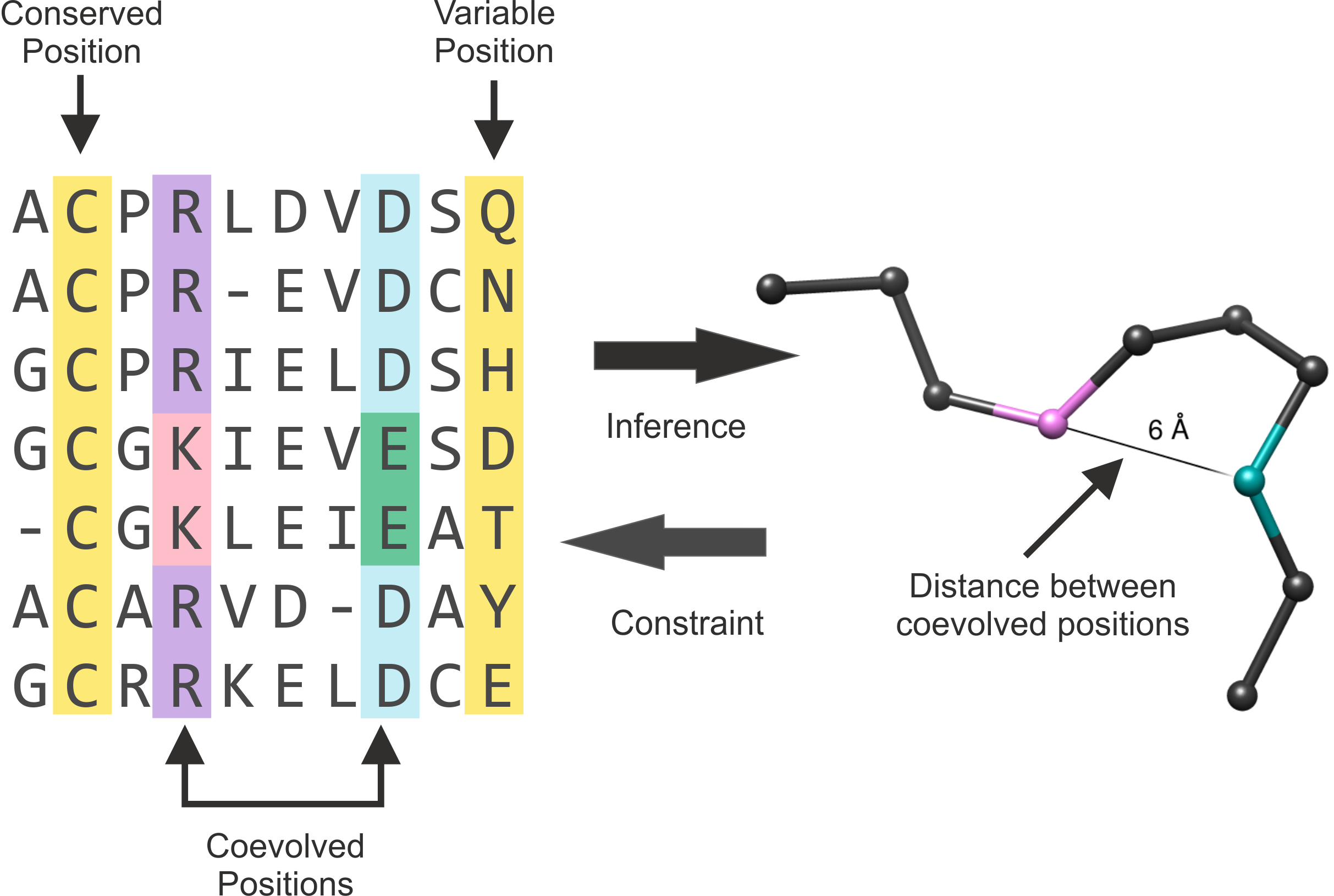 | |
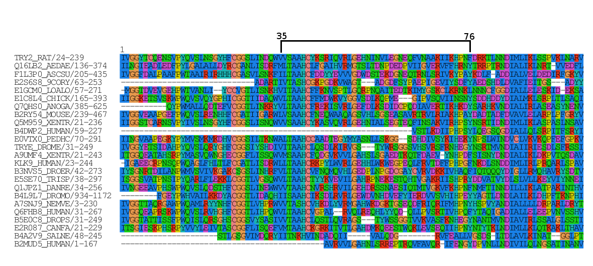
Figure 1. Representation of a MSA and the alpha-carbon structure of one protein of the alignment. Conserved and variable positions are highlighted in yellow. The positions that coevolved are
highlighted in purple and light blue. The residues within these positions where change occurred are shown in pink and green. The arrows (middle) represent the interrelation of coevolution and structural
information. This Figure is an adaptation of Figure 1 of (Marks et al., 2011). |
Mutual Information is a measurement of the uncertainty reduction for a MSA of homologous proteins. The MI between two positions (two columns in the MSA) reflects the extent to which knowing the
amino acid at one position allows us to predict the amino acid identity at the other position.
Motivated by these observations, a network composed of the residues is defined, where nodes are residues and links are set when the coevolutionary interaction strengths between residues are
sufficiently large.
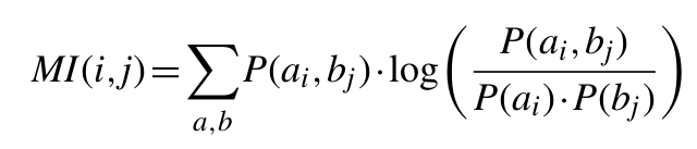
The MI between two positions in an MSA is given by the relationship:
Where P(ai, bi) is the frequency of amino acid a occurring at position i and amino acid b occurring at position
j in the same sequence, P(ai) is the frequency of amino acid a at position i and P(bj) is the frequency of amino acid
b at position j. In all cases MSAs were gap trimmed to remove positions with gaps in a reference sequence. In addition, all positions with > 50% gaps, as well as sequences covering <50% of the reference sequence length were removed. Unlike other methods, with this procedure we allow gaps to occur. Residue frequencies in positions with gaps are inferred from the count of the remaining observed pairs (keep in mind that positions with more than 50% of gaps are excluded from calculations).
We introduced a very simple correction for low number of sequences. The amino acid frequencies, P(a, b), are normalized from N(a,b), the number of times an amino acid pair (a, b) is observed at positions i and j in the MSA. From N(ai, bi), P(ai, bj) is calculated as (λ + N(ai, bi))/N, where:
It is clear that for MSAs of limited size, a large fraction of the P(ax, by) values will be estimated from a very low number of
observations, and their contribution to MI could be highly noisy. To deal with such low counts, the parameter λ was introduced. The initial value for the variable N(ai, bj) = λ is set for all amino acid pairs. Only for MSAs with a small number of sequences, where a large fraction of amino acid pairs
remain unobserved, will λ influence the amino acids occupancy calculation. For large MSAs, most amino acid pairs will be observed at least once, and the influence of λ will be minor.
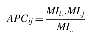
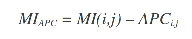
Also, the APC correction of Dunn et. al (2008) is applied:
Where MIi. is the average MI value of position i to all other positions in the MSA, and MI.. is the average MI value over all pairs of positions in the MSA.
Furthermore, MSAs will often suffer from a high degree of unnatural sequence bias and redundancy, as a result of multiple-strain sequencing and biased selection of sequenced species. It was
therefore expected that sequence clustering would improve the accuracy of the MI calculation. A Hobohm 1 algorithm (Hobohm et al., 992) is used to define sequence clusters, assigning to each sequence
within a given cluster a weight corresponding to one divided by the number of sequences in that cluster.
Finally, a Z-score transformation to allow for comparison across different families is applied. All prediction scores are compared with a distribution of prediction scores obtained from a large set
of randomized MSAs. The Z-score is then calculated as the number of standard deviations that the observed MI value falls above the mean value obtained from the randomized MSAs.
Although the MI is calculated between pairs of residues, groups of residues that coevolve form a network. MI networks are defined as graphs G(N,E), where nodes (set N) were defined as positions in
the MSA of a family (i.e. the columns of the MSA) and edges (set E) are defined between any pair of nodes with MI>6.5 (interactively modifiable in the server). These networks are called MI Networks
(MINs).
Distance networks (DN) are defined for the reference protein of every MSA as graphs G'(N',E'), where nodes (set N') are the residues (i.e residue numbering) of the reference protein, and edges (set
E') are defined between pairs of residues at a distance shorter than 5Å.
The basis for calculating Mutual Information for a group of homologous proteins is a Multiple Sequence Alignment (MSA). A MSA consists of sequences of proteins aligned
utilizing software dedicated to this task such as Clustal, T-Coffee and Muscle, among others. The server accepts as input MSAs in FASTA format (which is a standard format to store sequences).A sequence in FASTA format
begins with a single-line description, followed by lines of sequence data (for proteins, amino acids in one letter code). The description line is distinguished from the sequence data by a greater-than
(">") symbol at the beginning. The word following the ">" symbol is the identifier of the sequence, and the rest of the line is the description (both are optional). There should be no space between the
">" and the first letter of the identifier. This format is valid for aligned and unaligned sequences. If the sequences are aligned, they can also contain gaps as dashes ("-") or dots (".").
MSAs can be downloaded from different databases (e.g. Pfam, Cath, among others), and the server provides the option to automatically load a Pfam alignment.
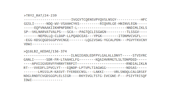 |
Fasta format of the first two aligned sequences in a MSA. In this case, each identifier is composed by an Uniprot Entry Name, followed by two numbers, specifying the portion
of the full sequence it contains. This composed sequence identifier is used in the PFAM domain alignments. |
The construction of the MSA is crucial and decisive to the calculation of Mutual Information (MI). Collecting sequences and aligning them can be a demanding task.
For optimal performance the MSA should be large and diverse. MSAs with > 400 sequences (or 400 clusters of sequences) < 62% identical show good predictive performance values (AUC > 0.75).
(Marino Buslje et al, 2009). These values are usually achieved by having ~2000 sequences in the alignment.
Keep in mind that that covariation and coevolution are not identical. Covariation signal is made up of phylogeny, structure, function, interactions, and stochastic components (Atchley et al. Mol Biol Evol 2000). High MI scores are not proof of coevolution, they are suggestive of it. MI scores can be misleading if sequences are not collected properly and alignments not built correctly.
PFAM is a large collection of protein domain families. Each family is represented by multiple sequence alignments and hidden Markov models. In general, the number of sequences and the quality of the
alignments in the PFAM database is good enough for calculating Mutual Information.
If you do not have a MSA or don't know how to make one, we can suggest one by clicking in the "I don't have a MSA, help me get one" link. Based on the
Uniprot name of a protein of interest or by uploading a sequence, we can suggest a PFAM domain MSA.
The reference sequence is your sequence of interest in the alignment. Selecting a reference sequence will remove all columns of the MSA (Multiple Sequence Alignment) where a gap is found in the selected sequence. The reference sequence will be left unchanged. In addition
sequences covering <50% of the reference sequence length are removed.
For selecting a reference sequence, you have to write the FASTA identifier in the input box provided. Don't worry if you do not remember the exact name, the input box has an autocomplete
feature, based on the identifiers in your MSA.
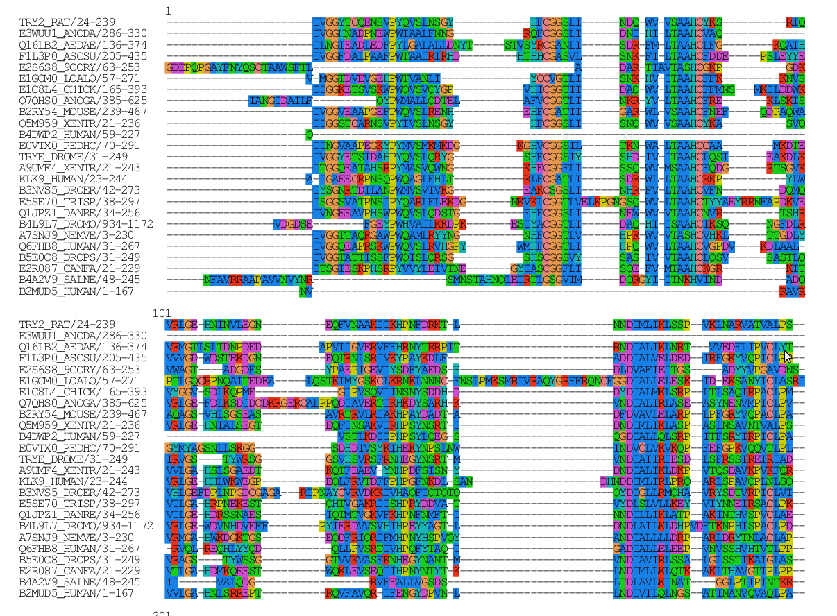 | 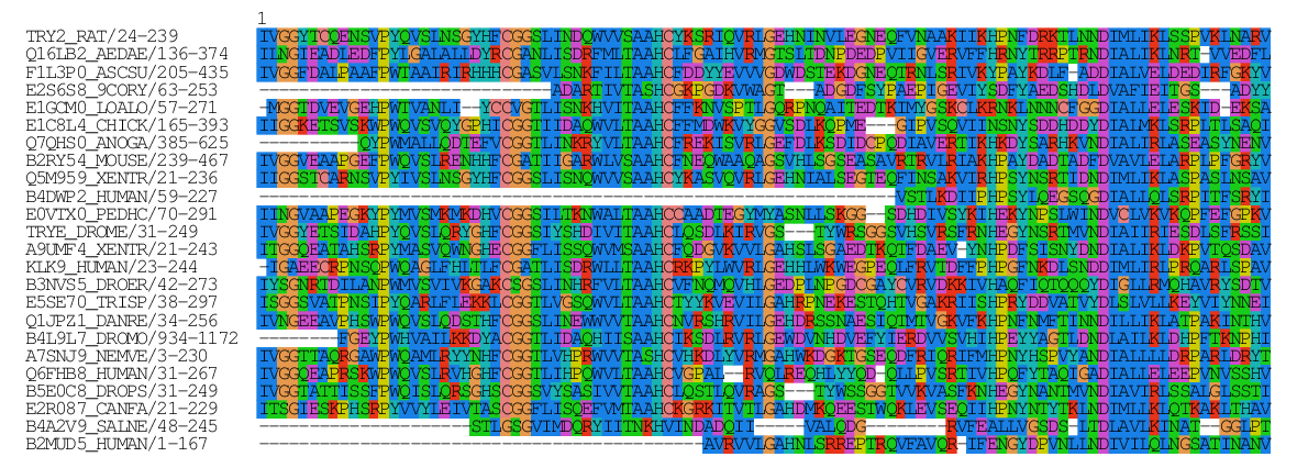 |
Gapped, original alignment | Gap stripped alignment, using the first sequence as reference |
If no reference sequence is selected, the labels in some of the results will still appear associated to the first sequence in your MSA, but gap removal will not occur. Also, structural data won't be
available since there is no reference sequence for the structure to be aligned to.
Some protein sequences have a known 3D structure, available in the PDB database. If available, we can use this structural information to show the Mutual Information relationships between positions
of your sequence of interest (i.e, your reference sequence) in a 3D structure. For this, the sequence in the PDB will be aligned to your reference sequence using a waterman-smith algorithm. Positions from the reference sequence (and hence, from the MSA) that cannot be aligned to the PDB sequence, will not be available in the results (be careful!). You can check the PDB-refseq alignment in the '3D structure' tab in the interactive network results.
PDB structure files are specified by a 4-letter PDB id. You can input the PDB id or upload your own PDB file. After this, you will be required to select which chain of the
model you want to align to your reference sequence. For structures obtained with RMN techniques, the first model is selected as default, then you will be asked to specify a chain.
 |
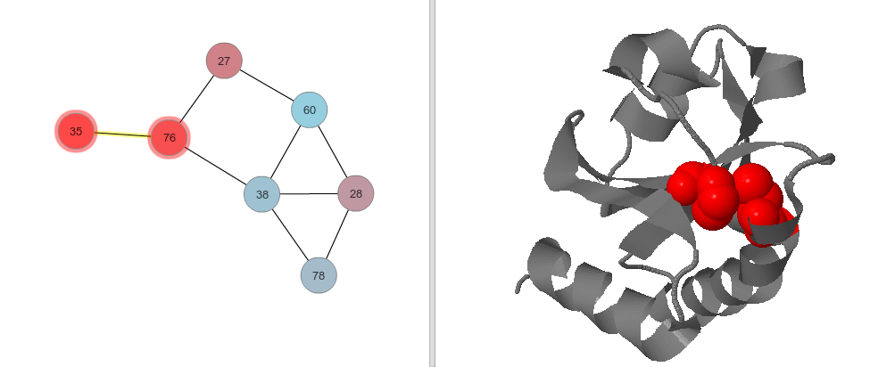 |
Mutual Information relationship between positions 35 and 76 (left), displayed in a PDB structure (right) for the reference sequence (first sequence in alignment). |
When dealing with biological data, MSAs will often suffer from a high degree of unnatural sequence bias and redundancy, as a result of multiple-strain sequencing and biased selection of sequenced
species. It was therefore expected that the sequence clustering would improve the accuracy of the MI calculation. In (Marino Buslje et al, 2009) is shown the use of a Hobohm 1 algorithm (Hobohm et al, 1992) to define sequence clusters, and assign each sequence within a given cluster a weight
corresponding to one divided by the number of sequences in the cluster. In this work clusters were defined at a sequence identity threshold of 62%.
It is also clear that for MSAs of limited size, a large fraction of the P(ax, by) values will be estimated from a very low number of
observations, and their contribution to MI could be highly noisy. To deal with such low counts, a parameter λ was introduced. The initial value for the variable N(ai, bj) = λ is set for all amino acid pairs. We tested a range of λ values 0 - 0.2 in steps of 0.01. The maximal performance was
achieved for a value of λ equal to 0.05, but similar results were obtained in the range 0.025 - 0.075. That means that all possible amino acids pairs will be observed at least 0.05 times
(λ). Only for MSAs with a small number of sequences, where a large fraction of amino acid pairs remain unobserved, λ will influence of the amino acids occupancy calculation. For large
MSAs, most amino acid pairs will be observed at least once, and the influence of λ will be minor.
By default columns in the MSAs with >50% of gaps are not allowed in calculations. Users can adjust this value in the 'Advanced Options'. Unlike other methods, this procedure allows gaps to occur.
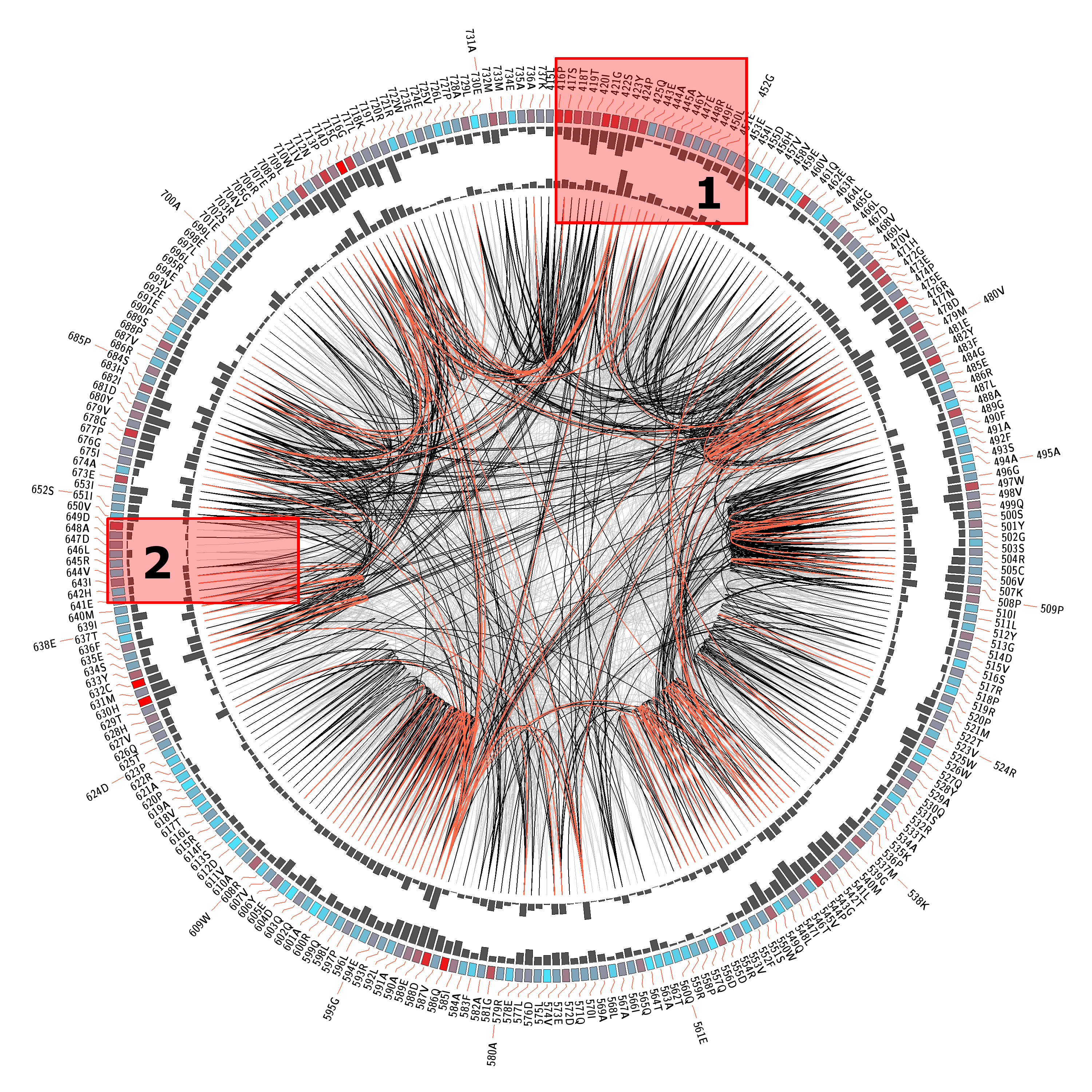
MI Circo is a sequential circular representation of the MSA and the information it contains. The information of each circle from outer to inner is the following: labels in the first (outer) circle
indicate the alignment position and the amino acid code of the reference sequence. The colored square boxes of the second circle indicate the MSA position conservation (highly conserverd positions are
in red, while less conserved ones are in blue).The third and fourth circles show the Proximity MI (pMI) and Cumulative MI (cMI) as histograms, facing inwards and outwards respectively. In the center of the circle lines can be observed, that connect pairs of
positions with MI greater than 6.5 (Marino Buslje et al, 2009).
 |
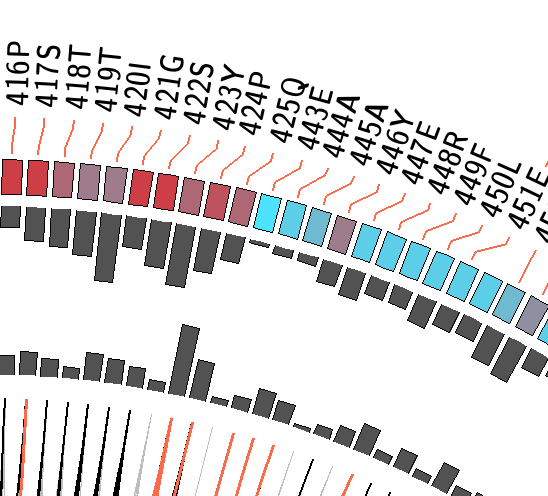 | 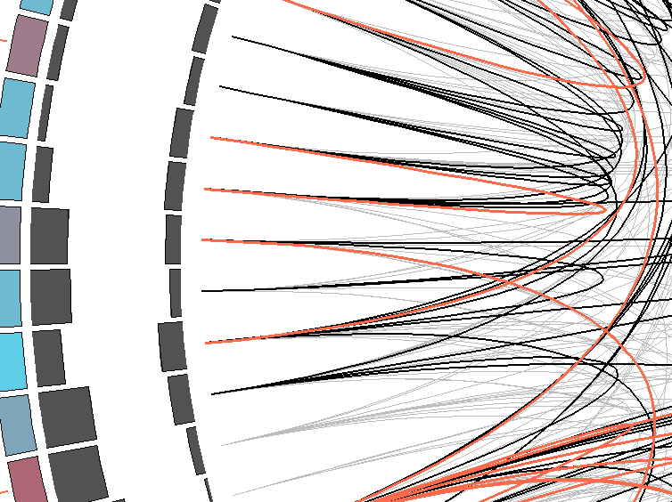 |
1) Contiguous positions in the MSA with information about conservation (red and blue rectangles),
cumulative MI (histogram facing outwards) and proximity MI (histogram facing inwards) |
2) Mutual information relationship between MSA positions. Red edges represent the top 5%, black ones are between 70% and 95%, and gray edges account for the remaining 70%. |
Besides the Circo representation, the same data is displayed in a network layout. Each node represents a position in the MSA and lines between nodes (edges) represent a significative mutual information value (> 6.5). Node color represents site conservation, red is for very conserved sites while blue is for less conserved sites. In case a PDB was supplied, distance network will also be shown with position at < 5 Å.
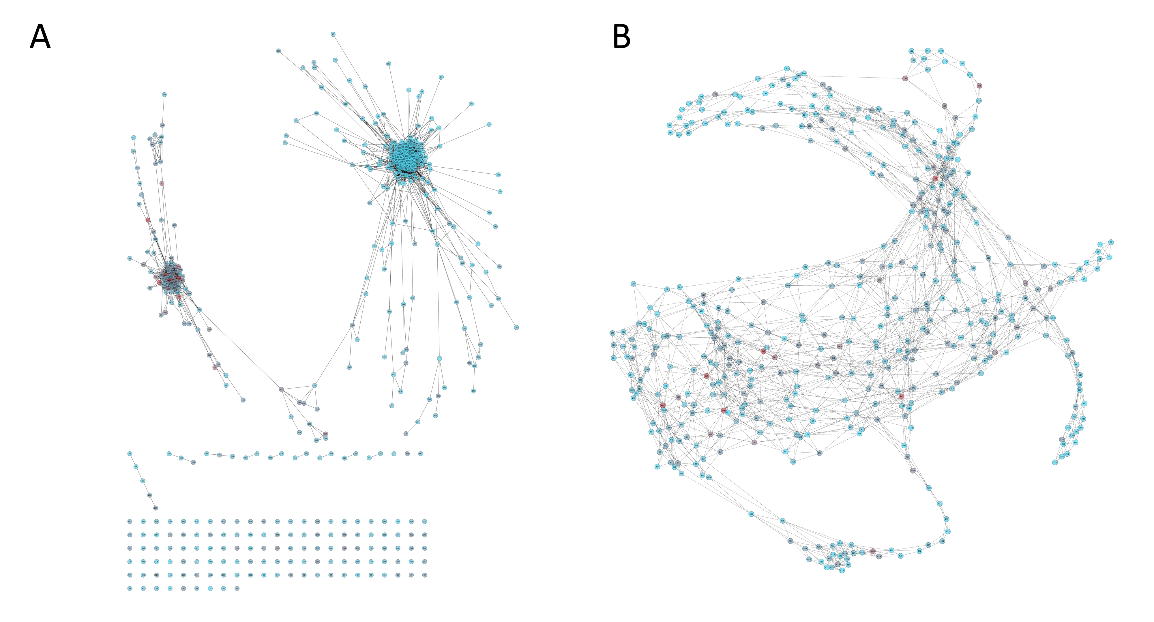 |
(A) Mutual Information network and (B) Distance network for VL1_HPV protein family (PF00500) |
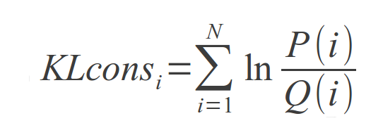
Conserved residues in protein families usually determine positions that play important biological or structural roles. Several metrics exist for measuring conservation in protein sequences. One of such,
the Kullback-Leibler (KL) divergence, is used for such purpose in this web toolkit. For each column of the Multiple Sequence Alignment, the KL conservation is calculated as
where P(i) is the frequency of aparition of aminoacid i in that position and Q(i) is the background frequency of the amino acid in nature (Cover and Thomas, 1991) calculated using an amino
acids background frequency distribution obtained from the Uniprot database.
cMI is a mutual information score per position that characterizes the extent of mutual information "interactions" in its physical neighbourhood. This score is calculated as the sum of MI values
above a certain threshold for every amino acid pair where the particular residue appears. This value defines to what degree a given amino acid takes part in a mutual information network.
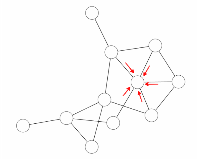 |
| The cMI score is obtained by adding to each node the MI value of the edges it has. |
pMI score is a value for each position as the sum of cMI of all the positions within a certain physical distance when mapped in a 3D structure. The distance
between each pair of residues in the structure was calculated as the shortest distance between any two atoms different from H belonging to each of the two positions. The threshold distance to be
included in each residue pMI score in the server is 5Å as this value approximates the upper limit for attractive London-van der Waals forces.
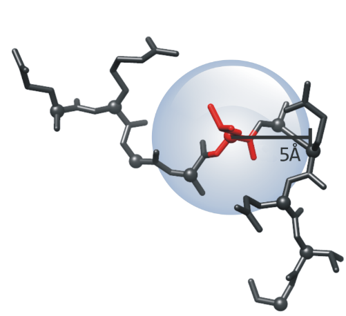 |
| The pMI score is the sum of cMI values of residues at 5Å. |
Help - Cytoscape
This section is intended to aid you in taking full advantage of the interactive web toolkit for visualizing, networks, structura, and alignment data.
The table shown displays the data associated to the selected nodes. Each node is displayed in a table row, where Label or ID is shown, with its conservation, Cumulative MI, and Proximity MI values (if a pdb structure was supplied). Shift-clicking nodes add the selected node data to the table, and removes data if the node was deselected. Drag-selection is also possible.
Clicking on the table headers is possible to sort the data displayed at any time.
When selecting a single node, an histogram will be displayed. It represents the relative aminoacid frequencies that correspond to that column in the Multiple Sequence Alignment.
The sum of all frequencies add up 1. A color code is using for illustrating different types of aminoacid. For example, a node may not be very conserved at all, but the histograms shows
that only hydrophobic aminoacids are encountered in that position.
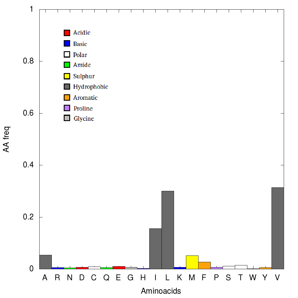 |
Histogram of aminoacid frequencies for a single column of the MSA. Conservation for this position is not considerably high, but only hydrphobic aminoacids are
found. |
If more than one node is selected, the sequence logo representation for the selected nodes will be displayed. The Y-axis describes the amount of information in bits while the X-axis shows the
position in the alignment. Each logo consists of stacks of symbols, one stack for each position in the sequence. The overall height of the stack indicates the sequence conservation at that position,
while the height of symbols within the stack indicates the relative frequency of each amino at that position. High stacks represents conserved positions and small stacks represents variable positions.
Colors represent characteristics of each aminoacid: in red are aminoacids D and E, green for N, Q, S, G, T and Y, in blue are H, K and R, and the rest are in black (A, V, I, L, M, F, W). The image is created using Seq2Logo.
Information regarding edges will be displayed in a table format when one or more are selected. Two types of edges can be found: Mutual Information (MI) edges and Distance edges. The later will
only be available if a PDB structure was supplied. For each node, the Label or ID and the value will be shown. The Label is composed of the node labels that are joined by the edge, along with the type
of edge. For example, an MI edge that joins nodes 20 and 30 will have a label like "20 (MI) 30".
the submitted PDB structure is displayed in the Jmol applet. To map the network nodes into the structure, an alignment between the PDB sequence and the MSA reference sequence was done. So when a
node in the network is selected, the corresponding residue in the structure is highlighted in red. Since PDB sequence may differ from the reference sequence (or perhaps it is a completely different
one), gaps can be introduced in the alignment, and no relationship can be established for those positions. That's why it is very important to choose a PDB that can be related to the reference sequence.
The buttons "Select chain X" and "Select Aligned Section" shown below the Jmol Applet allow to display either the complete PDB chain or the PDB-reference sequence aligned region. The checkbox on the left allows to show/hide the selected residue labels and numbers.
Besides selecting nodes in the network to highlight its structual counterpart, this method is impractical when trying to select contiguous residues or when trying to find a specific position. To this end, the "Select Nodes by Label" feature is available. Introducing the node labels is possible to select those nodes, and at the same time the corresponding residues in the
structure. Comma-separated node labels are accepted (e.g 123,129,150,..) or a range of nodes separated with a mid-hyphen (e.g 120-140). Combinations of both formats are accepted separated by commas
and no white spaces (e.g 74,92,115-130,25,40-50)
Selection of edges can be done specifying the pair of nodes conected by an edge. For example, if nodes 25 and 50 are connected by an edge, to select it by label one needs to enter the node label id separated by a middle hyphen (eg, 25-50). Comma-separated pairs of node labels are also accepted (e.g 25-50,129-135,150-170,...).
Multiple structural regions or networks groups can be saved using different settings, so different properties can be shown at once. First, a selection must be made (by clicking on the network, or
selecting nodes by label). An identifier for the selection is required then. For example, if we found a group of nodes of interest, we can call it "Cluster 1". A color can be selected from the drop
-down list, and a spatial representation for the atoms in the structure (Cartoon, VDW radius, ball and sticks, sticks, lines). Clicking on "Save" will create a new element in the "Shown" list with its
name and the chosen color. Elements from the "Shown" list can be moved to the "Hidden" list, so they won't be displayed in the structure. One or more items can be selected at the same time to be moved
, deleted, or re-selected. The last action may sound odd, since we are dealing with saved selections. The problem is that the saved selections are only persistent and shown in the PDB structure, but
the selected nodes in the network are lost. Selecting one or more options from the Shown or Hidden lists and clicking "Select on the network" will recover those node selections
An edge filter allows to hide or show edges according to one of their properties. There are two kinds of edge filters: Mutual information filter and a Distance filter. The Mutual Information (MI)
filter works by moving a slider. It has two limits, a lower and an upper one. The edges with a MI value between these two limits will be displayed, while those that fall outside this range
will remain hidden. On the other hand, the distance filter works only by showing or hidding distance edges. This edges correspond to residues which have any of their heavy atoms at less than 5 Å.
Furthermore, an additional filter can be applied to only show distance edges for those nodes that have at least one MI edge associated. When necessary, if the network is rescaled, or filtered in any other way, the "Update" button should be used to re-apply this behaviour (to display distance edges for nodes with MI)
Edges can also be filtered depending on the sequence distance between positions. For example, edges between nodes less than 3 positions apart can be excluded from the graph. This can be helpful if the user wants to exclude (or viceversa) secondary structure mutual information signals. The filter works by hidding nodes more than n values from any residue i in the network.
Node filters, like edge filter, allow for selectively showing or hidding nodes based on their properties. By moving the sliders, a range of values can be selected for which the nodes that satisfy
the restriction will be shown and the rest will be hidden. There are 2 basic properties for all nodes, Conservation and Cumulative MI. The first one is based on the Multiple Sequence Alignemnt column that correspond to that node. One more type of property pMI can be used if a PDB structure was provided.
Based on the network topology, "First Neighbours" are those that, relative to a node or a group of nodes, are the first nodes to get "visited" when travelling along the edges of the selected nodes. By selecting one or more nodes, this tool finds its first neighbours
Similar to the first neighbour algorithm, we call the "Associated Maximal Subnetwork" to the group of nodes that, starting from one or more nodes, can be visited by travelling along their edges. In other words, it finds the whole network containing the selected nodes. It is a recursive implementation of the first neighbours algorithm.
When several nodes are selected, either by clicking in the network or by entering node labels, it is useful to save the selection for future analysis. To do this, first made a selection and enter an
identifier, such as "Group 1”. Once it is done, a new entry will appear in the "Saved Selections" list. One or more entries can later be selected and by pressing the "Select" button, they will be
selected on the network. The same way, selections can be removed using the "Delete" button.
Networks can be exported in six available formats, ranging from images to network specific formats.
GraphML (GML):
GraphML is a XML-based file format used for graphs.More information can be found here
eXtensible Graph Markup and Modeling Language (XGMML):
Another graph XML-based format, which can be loaded onto Cytoscape's Desktop version.
Scalable Vector Graphic (SVG) :
Vectorized image, can be scaled without losing resolution.
Portable Document Format (PDF):
PDF file with network image.
Portable Network Graphic (PNG):
Widely used image format.
Simple Network File (SIF):
Plain text file format.
Network layouts describe the way and the principles in which nodes, edges and the disposition of them will be visualized
Circular Layout:
Nodes are arranged in a circle with straigth edges connecting them Radial Layout:
A node is picked to be central and its first neighbours are arranged around it. New nodes continue to make new layers around the central node.
Tree Layout :
A tree-based view features a node at the top of the hierarchy, with nodes descending to become leaves of the tree
Force Directed Layouts:
Force directed layouts are done by simulating the network as a physical system, where nodes are balls of a constant mass joined by springs (edges) with a certain elastic constant. The system is iterated until it becomes stable or reaches a limited number of iterations.
Unweighted
In this case all springs have the same elastic constant.
Weighted
For weighted force directed layouts, the elastic force of each spring is proportional to the value that edge contains. For example, for a Mutual Information force directed layout, edges with high MI will have greater force and hence have a shorter length. When one edge attribute is selected as weight, the other attributes remain unweighted.
Conservation
Kullback-Leibler conservation score is mapped from red to cyan, where red corresponds to high scores (very conserved) and cyan to low scores
Cumulative MI
Cumulative MI score is mapped from yellow (low score) to purple (high score)
Proximity MI
Proximity MI score is mapped from green (low score) to red (high score)
Secondary Structure
When a PDB structure is available, pink nodes represent a helix structure, yellow maps beta-sheet structures, blue corresponds to turns and white to random coils. The mapping is done using DSSP ( ref )